import polars as pl
import seaborn as sns
import matplotlib.pyplot as plt
from mplstyle import mplstyle_from_brand
from brand_yml import Brand

from pyprojroot.here import here

mplstyle_from_brand(here("_brand.yml"))Predicting Incidence of Diabetes
Machine Learning
Random Forest
markdown text
Now get the data
df = pl.read_csv(here("projects/diabetes/diabetes.csv"))

print(df)
shape: (768, 9)
┌─────────────┬─────────┬───────────────┬───────────────┬───┬──────┬───────────────┬─────┬─────────┐
│ Pregnancies ┆ Glucose ┆ BloodPressure ┆ SkinThickness ┆ … ┆ BMI ┆ DiabetesPedig ┆ Age ┆ Outcome │
│ --- ┆ --- ┆ --- ┆ --- ┆ ┆ --- ┆ reeFunction ┆ --- ┆ --- │
│ i64 ┆ i64 ┆ i64 ┆ i64 ┆ ┆ f64 ┆ --- ┆ i64 ┆ i64 │
│ ┆ ┆ ┆ ┆ ┆ ┆ f64 ┆ ┆ │
╞═════════════╪═════════╪═══════════════╪═══════════════╪═══╪══════╪═══════════════╪═════╪═════════╡
│ 6 ┆ 148 ┆ 72 ┆ 35 ┆ … ┆ 33.6 ┆ 0.627 ┆ 50 ┆ 1 │
│ 1 ┆ 85 ┆ 66 ┆ 29 ┆ … ┆ 26.6 ┆ 0.351 ┆ 31 ┆ 0 │
│ 8 ┆ 183 ┆ 64 ┆ 0 ┆ … ┆ 23.3 ┆ 0.672 ┆ 32 ┆ 1 │
│ 1 ┆ 89 ┆ 66 ┆ 23 ┆ … ┆ 28.1 ┆ 0.167 ┆ 21 ┆ 0 │
│ 0 ┆ 137 ┆ 40 ┆ 35 ┆ … ┆ 43.1 ┆ 2.288 ┆ 33 ┆ 1 │
│ … ┆ … ┆ … ┆ … ┆ … ┆ … ┆ … ┆ … ┆ … │
│ 10 ┆ 101 ┆ 76 ┆ 48 ┆ … ┆ 32.9 ┆ 0.171 ┆ 63 ┆ 0 │
│ 2 ┆ 122 ┆ 70 ┆ 27 ┆ … ┆ 36.8 ┆ 0.34 ┆ 27 ┆ 0 │
│ 5 ┆ 121 ┆ 72 ┆ 23 ┆ … ┆ 26.2 ┆ 0.245 ┆ 30 ┆ 0 │
│ 1 ┆ 126 ┆ 60 ┆ 0 ┆ … ┆ 30.1 ┆ 0.349 ┆ 47 ┆ 1 │
│ 1 ┆ 93 ┆ 70 ┆ 31 ┆ … ┆ 30.4 ┆ 0.315 ┆ 23 ┆ 0 │
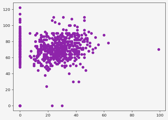
└─────────────┴─────────┴───────────────┴───────────────┴───┴──────┴───────────────┴─────┴─────────┘fig, ax = plt.subplots()
ax.scatter(
x = df["SkinThickness"],
y = df["BloodPressure"]
)